Analyzing high-throughput FACS assays with R
Note: Updated March 28, 2022 to reflect updated packages. Previous tutorial version is here.
Introduction
Analysis of flow cytometry data with R may seem daunting at first but I highly recommend it to anyone performing mid- or high-throghput FACS-based assays. I frequently run experiments in 96-well formats with hundreds of samples (this obviously requires a plate reader on your FACS machine). Even if you only look at very few markers, traditional flow analysis software like FlowJo doesn’t handle large numbers of samples well. It’s slow, prone to crashing and exporting large plots is painful. This is where flow cytometry analysis in R does a great job. There are multiple R packages for flow cytometry data analysis. The two packages I am using in this tutorial and which I highly recommend are:
Both have great documentation and I suggest you work through their vignettes to get you started with flow analysis in R. The following tutorial assumes that you have some knowledge of flow cytometry data analysis (such as basic gating operations) and familiarized yourself with the basics of flowCore datastructures and functions.
In the example analysis below, I am looking at the fraction of GFP
positive cells in a 96-well plate. Each well has been infected with a
different GFP-tagged gRNA. In the actual experiment, I then look at the
fraction of GFP positive cells over time to see which gRNAs drop out.
For now, we’ll just be looking at one timepoint / dataset.
Because I am only looking at one marker, no compensation is required.
Note also, that I am not transforming the data (as suggested by the
flowCore vignette). Instead, I use the scale function of ggcyto
(e.g. scale_x_flowJo_biexp) which I find much more convenient.
If you’d like to follow along, you can download the example data here.
Load required libraries
library(flowCore)
library(ggcyto)
library(tidyverse)
library(knitr)
Read and format .fcs data
The read.flowSet allows you to read many .fcs at once. The resultant
flowSet object will store the data from all these .fcs files.
fs <- read.flowSet(path = "../../downloads/2020-07-08-FACS-data//",pattern = ".fcs",alter.names = T)
Sample information (aka phenotypic data) such as sample names can be
accessed with the pData function. The default sample names are not
very useful. So, let’s extract the well ID from the sample name (this
will make things easier later on).
pData(fs)[1:3,]
## [1] "Specimen_001_B10_B10_009.fcs" "Specimen_001_B11_B11_010.fcs"
## [3] "Specimen_001_B2_B02_001.fcs"
pData(fs)$well <- gsub(".*_.*_(.*)_.*.fcs","\\1",sampleNames(fs)) # extract well from name and add new 'well' column
pData(fs)[1:3,]
##                                                      name well
## Specimen_001_B10_B10_009.fcs Specimen_001_B10_B10_009.fcs  B10
## Specimen_001_B11_B11_010.fcs Specimen_001_B11_B11_010.fcs  B11
## Specimen_001_B2_B02_001.fcs   Specimen_001_B2_B02_001.fcs  B02
The default channel names on most FACS machines are useless and changing them there is often tedious. On our BD FACS Canto II, for example, the [405|450/50] channel is named “Pacific.Blue.A” and the [488|530/30] is named “FITC.A” - irrespective of the fluorphore you are actually reading. Below is a quick and simple way to change the channel names for the entire flowSet. This makes coding easier and will result in proper axis labels in your plots.
colnames(fs)
## [1] "FSC.A"          "FSC.H"          "FSC.W"          "SSC.A"
## [5] "SSC.H"          "SSC.W"          "FITC.A"         "Pacific.Blue.A"
## [9] "Time"
colnames(fs)[colnames(fs)=="FITC.A"] <- "GFP"
colnames(fs)[colnames(fs)=="Pacific.Blue.A"] <- "BFP"
To be able to add gates, the flowSet has to be transformed to a
GatingSet object with the GatingSet function
gs <- GatingSet(fs)
Set singlet gate
There are automatic singlet gating commands available,
e.g. flowStats::gate_singlet. However, I generally find manual gating
more reliable. As with all gating steps below, setting the gates can be
tedious in R as opposed to interactive gating with FlowJo. However, if
you usually use similar cells or cell lines and keep the voltage
settings on your machine constant, you really only have to set these
gates once. After that, all you may have to do is tweak the gates a
little. The basic steps I take for each of the gatings below are:
- define the gate
- check the gate in a plot (before adding it to the gating set)
- if the gate seems right, add / apply it to the gating set
- recompute the gatingSet to have statistics available
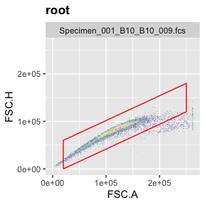
g.singlets <- polygonGate(filterId = "Singlets","FSC.A"=c(2e4,25e4,25e4,2e4),"FSC.H"=c(0e4,12e4,18e4,6e4)) # define gate
ggcyto(gs[[1]],aes(x=FSC.A,y=FSC.H),subset="root")+geom_hex(bins = 200)+geom_gate(g.singlets)+ggcyto_par_set(limits = "instrument") # check gate
add(gs,g.singlets) # add gate to GatingSet
recompute(gs) # recompute GatingSet
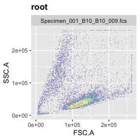
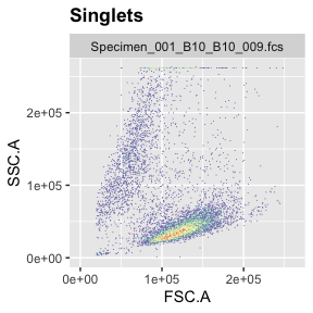
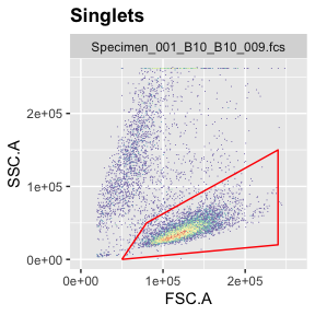
If you want to check where the singlets you filtered out show up in FSC vs SSC (the plot that is typically used to remove debris or gate live cells), you can do this by setting different subets in the ggcyto command (‘root’ or ‘Singlets’).
ggcyto(gs[[1]],aes(x=FSC.A,y=SSC.A),subset="root")+geom_hex(bins = 200)+ggcyto_par_set(limits = "instrument")
ggcyto(gs[[1]],aes(x=FSC.A,y=SSC.A),subset="Singlets")+geom_hex(bins = 200)+ggcyto_par_set(limits = "instrument")
 Now comes the fun part
where R works so much better than FlowJo: plotting the data for all
samples at once. This is based on ggplot’s
Now comes the fun part
where R works so much better than FlowJo: plotting the data for all
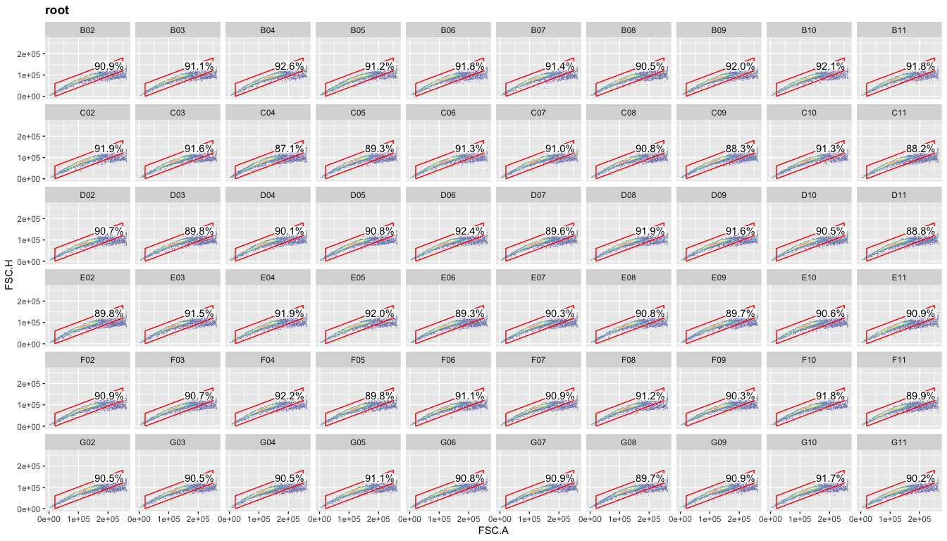
samples at once. This is based on ggplot’s facet_wrap command
(included by default in ggcyto when using even if you don’t explicitly
call that command). If we now use the ‘well’ column with facet_wrap,
we’ll get meaningful titles for each plot. Although you might not use
this overview plot for any kind of publication (espcially not something
boring like your singlet gate), this kind of plot allows you to
immediately spot any issues with certain samples (dead cells, clumped
cells, technical errors with your FACS machine). Thus, I recommend
generating these overview plots at each gating step.
ggcyto(gs,aes(x=FSC.A,y=FSC.H),subset="root")+geom_hex(bins = 100)+geom_gate("Singlets")+
  geom_stats(adjust = 0.8)+ggcyto_par_set(limits = "instrument")+
  facet_wrap(~well,ncol = 10)
 ## Set live gate
Gating steps are as above. Differentiating live and dead cells solely
based on FSC/SSC works very well for the cells used here (OCI-LY7) but
may not work well for all kinds of cells.
g.live <- polygonGate(filterId = "Live","FSC.A"=c(5e4,24e4,24e4,8e4),"SSC.A"=c(0,2e4,15e4,5e4)) # define gate
ggcyto(gs[[1]],aes(x=FSC.A,y=SSC.A),subset="Singlets")+geom_hex(bins = 200)+geom_gate(g.live)+ggcyto_par_set(limits = "instrument") # check gate
add(gs,g.live,parent="Singlets") # add gate to GatingSet
recompute(gs) # recompute GatingSet
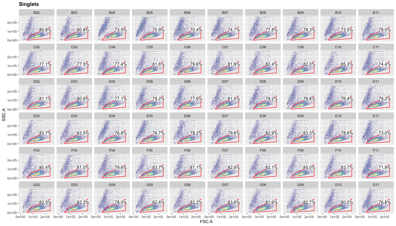
Again, you can plot the live gate for all samples.
ggcyto(gs,aes(x=FSC.A,y=SSC.A),subset="Singlets")+geom_hex(bins = 100)+geom_gate("Live")+
  geom_stats(adjust = 0.8)+ggcyto_par_set(limits = "instrument")+
  facet_wrap(~well,ncol = 10)
Set GFP+ gate
Because we are only looking at one channel (GFP) for the next gating step, we can now switch to density plots instead of the hex plots above. These are faster to generate, simpler to look at and need less storage.
g.gfp <- rectangleGate(filterId="GFP positive","GFP"=c(1000, Inf)) # set gate
ggcyto(gs[[1]],aes(x=GFP),subset="Live")+geom_density(fill="forestgreen")+geom_gate(g.gfp)+ggcyto_par_set(limits = "instrument")+scale_x_flowJo_biexp() # check gate

add(gs,g.gfp,parent="Live") # add gate to GatingSet
recompute(gs) # recalculate Gatingset
Now, we can look at the data we were looking for: the fraction of GFP positive cells in each well.
ggcyto(gs,aes(x=GFP),subset="Live",)+geom_density(fill="forestgreen")+geom_gate("GFP positive")+
  geom_stats(adjust = 0.1,y=0.002,digits = 1)+
  ggcyto_par_set(limits = "instrument")+scale_x_flowJo_biexp()+
  facet_wrap(~well,ncol = 10)

Get populations stats for downstream analysis
To get the data from each gating step from the GatingSet, we can use
the gs_pop_get_count_with_meta function (which conveniently also
retrieves all the metadata and sample names you might have added).
ps <- gs_pop_get_count_with_meta(gs)
We can now easily calculate the ‘percent of parent’ (a common metric in FACS analysis).
ps <- ps %>% mutate(percent_of_parent=Count/ParentCount)
ps %>% select(sampleName,well,Population,Count,ParentCount,percent_of_parent) %>% head() %>% kable
| sampleName | well | Population | Count | ParentCount | percent_of_parent |
|---|---|---|---|---|---|
| Specimen_001_B10_B10_009.fcs | B10 | /Singlets | 9211 | 10000 | 0.9211000 |
| Specimen_001_B10_B10_009.fcs | B10 | /Singlets/Live | 6770 | 9211 | 0.7349908 |
| Specimen_001_B10_B10_009.fcs | B10 | /Singlets/Live/GFP positive | 3467 | 6770 | 0.5121123 |
| Specimen_001_B11_B11_010.fcs | B11 | /Singlets | 9176 | 10000 | 0.9176000 |
| Specimen_001_B11_B11_010.fcs | B11 | /Singlets/Live | 7158 | 9176 | 0.7800785 |
| Specimen_001_B11_B11_010.fcs | B11 | /Singlets/Live/GFP positive | 4503 | 7158 | 0.6290863 |
I hope this tutorial was useful to you. Please feel free to email
me with any questions, comments or suggestions and I’ll be happy to post
them here.
info at jchellmuth.com
sessionInfo()
## R version 4.0.4 (2021-02-15)
## Platform: x86_64-apple-darwin17.0 (64-bit)
## Running under: macOS Big Sur 10.16
##
## Matrix products: default
## BLAS:   /Library/Frameworks/R.framework/Versions/4.0/Resources/lib/libRblas.dylib
## LAPACK: /Library/Frameworks/R.framework/Versions/4.0/Resources/lib/libRlapack.dylib
##
## locale:
## [1] en_US.UTF-8/en_US.UTF-8/en_US.UTF-8/C/en_US.UTF-8/en_US.UTF-8
##
## attached base packages:
## [1] stats     graphics  grDevices utils     datasets  methods   base
##
## other attached packages:
##  [1] knitr_1.38               forcats_0.5.1            stringr_1.4.0
##  [4] dplyr_1.0.8              purrr_0.3.4              readr_2.1.2
##  [7] tidyr_1.2.0              tibble_3.1.6             tidyverse_1.3.1
## [10] ggcyto_1.18.0            flowWorkspace_4.2.0      ncdfFlow_2.36.0
## [13] BH_1.78.0-0              RcppArmadillo_0.10.8.1.0 ggplot2_3.3.5
## [16] flowCore_2.2.0
##
## loaded via a namespace (and not attached):
##  [1] fs_1.5.2            matrixStats_0.61.0  lubridate_1.8.0
##  [4] RColorBrewer_1.1-2  httr_1.4.2          Rgraphviz_2.34.0
##  [7] tools_4.0.4         backports_1.4.1     utf8_1.2.2
## [10] R6_2.5.1            DBI_1.1.2           BiocGenerics_0.36.1
## [13] colorspace_2.0-3    withr_2.5.0         tidyselect_1.1.2
## [16] gridExtra_2.3       curl_4.3.2          compiler_4.0.4
## [19] rvest_1.0.2         graph_1.68.0        cli_3.2.0
## [22] Biobase_2.50.0      xml2_1.3.3          labeling_0.4.2
## [25] scales_1.1.1        hexbin_1.28.2       digest_0.6.29
## [28] rmarkdown_2.13      base64enc_0.1-3     jpeg_0.1-9
## [31] pkgconfig_2.0.3     htmltools_0.5.2     highr_0.9
## [34] dbplyr_2.1.1        fastmap_1.1.0       rlang_1.0.2
## [37] readxl_1.3.1        rstudioapi_0.13     farver_2.1.0
## [40] generics_0.1.2      jsonlite_1.8.0      magrittr_2.0.2
## [43] RProtoBufLib_2.2.0  Rcpp_1.0.8.3        munsell_0.5.0
## [46] S4Vectors_0.28.1    fansi_1.0.3         lifecycle_1.0.1
## [49] stringi_1.7.6       yaml_2.3.5          zlibbioc_1.36.0
## [52] plyr_1.8.7          grid_4.0.4          parallel_4.0.4
## [55] crayon_1.5.0        lattice_0.20-45     haven_2.4.3
## [58] hms_1.1.1           pillar_1.7.0        stats4_4.0.4
## [61] reprex_2.0.1        XML_3.99-0.9        glue_1.6.2
## [64] evaluate_0.15       latticeExtra_0.6-29 data.table_1.14.2
## [67] RcppParallel_5.1.5  modelr_0.1.8        png_0.1-7
## [70] vctrs_0.3.8         tzdb_0.2.0          cellranger_1.1.0
## [73] gtable_0.3.0        aws.s3_0.3.21       assertthat_0.2.1
## [76] xfun_0.30           broom_0.7.12        cytolib_2.2.1
## [79] aws.signature_0.6.0 ellipsis_0.3.2